library(epiUtils)
library(dplyr)
#>
#> Attaching package: 'dplyr'
#> The following objects are masked from 'package:stats':
#>
#>     filter, lag
#> The following objects are masked from 'package:base':
#>
#>     intersect, setdiff, setequal, union
library(ggplot2)
Introduction
The epiUtils package provides essential tools for
epidemiological analysis, including:
- Age-standardised rate calculations using direct standardisation
- Person-years computation for cohort studies with age stratification
- Built-in WHO 2000-2025 World Standard Population data
This vignette demonstrates the key functions using practical examples.
WHO World Standard Population
The package includes the WHO 2000-2025 World Standard Population data, which is commonly used for age standardisation in epidemiological studies.
# Load the WHO standard population data
data("who_2000_2025_standard_population")
# View the structure
head(who_2000_2025_standard_population)
#> # A tibble: 6 × 6
#> age_group who_world_standard_perc…¹ recalculation_to_add…² rounded_to_integers
#> <chr> <dbl> <dbl> <int>
#> 1 [0-5) 8.86 88569. 88569
#> 2 [5-10) 8.69 86870. 86870
#> 3 [10-15) 8.6 85970. 85970
#> 4 [15-20) 8.47 84670. 84670
#> 5 [20-25) 8.22 82171. 82171
#> 6 [25-30) 7.93 79272. 79272
#> # ℹ abbreviated names: ¹who_world_standard_percent,
#> # ²recalculation_to_add_to_1million
#> # ℹ 2 more variables: standard_for_seer_stat <int>, lower_age_limit <int>
# Summary of the data
str(who_2000_2025_standard_population)
#> tibble [21 × 6] (S3: tbl_df/tbl/data.frame)
#> $ age_group : chr [1:21] "[0-5)" "[5-10)" "[10-15)" "[15-20)" ...
#> $ who_world_standard_percent : num [1:21] 8.86 8.69 8.6 8.47 8.22 7.93 7.61 7.15 6.59 6.04 ...
#> $ recalculation_to_add_to_1million: num [1:21] 88569 86870 85970 84670 82171 ...
#> $ rounded_to_integers : int [1:21] 88569 86870 85970 84670 82171 79272 76073 71475 65877 60379 ...
#> $ standard_for_seer_stat : int [1:21] 88569 86870 85970 84670 82171 79272 76073 71475 65877 60379 ...
#> $ lower_age_limit : int [1:21] 0 5 10 15 20 25 30 35 40 45 ...Example 1: Calculate Person-Years by Age Strata
Let’s start with an example of calculating person-years for a cohort study. The default age groups now match the WHO 2000-2025 Standard Population, making it easy to calculate age-standardised rates.
# Create example cohort data
set.seed(123)
n_patients <- 100

cohort_data <- data.frame(
  patient_id = 1:n_patients,
  dob = as.Date("1950-01-01") + sample(-7300:7300, n_patients, replace = TRUE), # Random dates ±20 years
  study_entry_date = as.Date("2020-01-01") + sample(0:365, n_patients, replace = TRUE),
  study_exit_date = as.Date("2023-01-01") + sample(0:730, n_patients, replace = TRUE),
  event_status = sample(c(0L, 1L), n_patients, replace = TRUE, prob = c(0.8, 0.2))
)

# Ensure study_exit_date is after study_entry_date
cohort_data$study_exit_date <- pmax(
  cohort_data$study_exit_date,
  cohort_data$study_entry_date + 30
)

# View first few rows
head(cohort_data)
#>   patient_id        dob study_entry_date study_exit_date event_status
#> 1          1 1936-10-03       2020-10-12      2023-05-05            0
#> 2          2 1936-11-20       2020-06-07      2023-09-22            0
#> 3          3 1958-07-16       2020-04-30      2023-07-05            1
#> 4          4 1953-11-18       2020-04-19      2024-07-26            0
#> 5          5 1964-03-10       2020-06-06      2023-09-09            0
#> 6          6 1938-03-10       2020-03-04      2024-04-02            0

# Calculate person-years by 5-year age groups (default - matches WHO age groups)
person_years_who <- calculate_person_years_by_age_strata(cohort_data)
print("Person-years by WHO-compatible age groups:")
#> [1] "Person-years by WHO-compatible age groups:"
print(person_years_who)
#> # A tibble: 21 × 4
#>    age_group person_years events     n
#>    <fct>            <dbl>  <int> <int>
#>  1 [0-5)                0      0     0
#>  2 [5-10)               0      0     0
#>  3 [10-15)              0      0     0
#>  4 [15-20)              0      0     0
#>  5 [20-25)              0      0     0
#>  6 [25-30)              0      0     0
#>  7 [30-35)              0      0     0
#>  8 [35-40)              0      0     0
#>  9 [40-45)              0      0     0
#> 10 [45-50)              0      0     0
#> # ℹ 11 more rows

# Calculate person-years using custom age groups (10-year groups for comparison)
person_years_10yr <- calculate_person_years_by_age_strata(
  cohort_data,
  age_cut_points = c(0, 10, 20, 30, 40, 50, 60, 70, 80, 90, 100, 150)
)
print("Person-years by 10-year age groups:")
#> [1] "Person-years by 10-year age groups:"
print(person_years_10yr)
#> # A tibble: 11 × 4
#>    age_group person_years events     n
#>    <fct>            <dbl>  <int> <int>
#>  1 [0-10)             0        0     0
#>  2 [10-20)            0        0     0
#>  3 [20-30)            0        0     0
#>  4 [30-40)            0        0     0
#>  5 [40-50)            0        0     0
#>  6 [50-60)           77.0      5    24
#>  7 [60-70)          117.       7    39
#>  8 [70-80)           70.3      4    30
#>  9 [80-90)           74.7      1    28
#> 10 [90-100)          16.3      1     7
#> 11 [100+)             0        0     0
Example 2: Age-Standardised Rates with WHO Standard Population
Now let’s calculate age-standardised incidence rates using the WHO standard population. With the updated defaults, this is now much simpler since the age groups match automatically.
# Method 1: Direct calculation using WHO-compatible age groups (recommended)
# The default age groups now match WHO 2000-2025 Standard Population exactly

# First, let's verify the age groups match
print("Age groups from our person-years calculation:")
#> [1] "Age groups from our person-years calculation:"
print(levels(person_years_who$age_group))
#>  [1] "[0-5)"    "[5-10)"   "[10-15)"  "[15-20)"  "[20-25)"  "[25-30)"
#>  [7] "[30-35)"  "[35-40)"  "[40-45)"  "[45-50)"  "[50-55)"  "[55-60)"
#> [13] "[60-65)"  "[65-70)"  "[70-75)"  "[75-80)"  "[80-85)"  "[85-90)"
#> [19] "[90-95)"  "[95-100)" "[100+)"

print("WHO 2000-2025 Standard Population age groups:")
#> [1] "WHO 2000-2025 Standard Population age groups:"
print(who_2000_2025_standard_population$age_group)
#>  [1] "[0-5)"    "[5-10)"   "[10-15)"  "[15-20)"  "[20-25)"  "[25-30)"
#>  [7] "[30-35)"  "[35-40)"  "[40-45)"  "[45-50)"  "[50-55)"  "[55-60)"
#> [13] "[60-65)"  "[65-70)"  "[70-75)"  "[75-80)"  "[80-85)"  "[85-90)"
#> [19] "[90-95)"  "[95-100)" "[100+)"

print("Age groups match perfectly:",
      identical(levels(person_years_who$age_group), who_2000_2025_standard_population$age_group))
#> [1] "Age groups match perfectly:"

# Merge with WHO standard population data directly
asr_data_who <- person_years_who |>
  left_join(
    who_2000_2025_standard_population |>
      select(age_group, standard_pop = standard_for_seer_stat),
    by = "age_group"
  ) |>
  filter(person_years > 0) |>  # Ensure positive person-years for all groups
  select(age_group, events, person_years, standard_pop)

print("Data prepared for ASR calculation (direct WHO matching):")
#> [1] "Data prepared for ASR calculation (direct WHO matching):"
print(asr_data_who)
#> # A tibble: 9 × 4
#>   age_group events person_years standard_pop
#>   <chr>      <int>        <dbl>        <int>
#> 1 [50-55)        0         28.5        53681
#> 2 [55-60)        5         48.5        45484
#> 3 [60-65)        4         50.6        37187
#> 4 [65-70)        3         66.5        29590
#> 5 [70-75)        0         42.7        22092
#> 6 [75-80)        4         27.6        15195
#> 7 [80-85)        0         42.2         9097
#> 8 [85-90)        1         32.5         4398
#> 9 [90-95)        1         16.3         1500

# Calculate age-standardised rates
asr_result_who <- calculate_asr_direct(asr_data_who)
#> Warning: ! Found age groups with small/zero case counts:
#> • zero cases: [50-55), [70-75), [80-85) and < 5 cases: [60-65) (4 cases),
#>   [65-70) (3 cases), [75-80) (4 cases), [85-90) (1 case), [90-95) (1 case)
#> ℹ Small and zero case counts may produce unstable rate estimates
#> ℹ Consider wider age groups, longer follow-up, or data quality checks

print("Age-Standardised Rate Results (WHO age groups):")
#> [1] "Age-Standardised Rate Results (WHO age groups):"
print(paste("Crude rate:", round(asr_result_who$crude_rate_scaled, 2), "per 100,000"))
#> [1] "Crude rate: 5064.91 per 100,000"
print(paste("Age-standardised rate:", round(asr_result_who$asr_scaled, 2), "per 100,000"))
#> [1] "Age-standardised rate: 5223.67 per 100,000"
print(paste("95% CI:", round(asr_result_who$asr_ci_lower_scaled, 2), "-", round(asr_result_who$asr_ci_upper_scaled, 2)))
#> [1] "95% CI: 2953.5 - 9563.6"
print(paste("Total events:", asr_result_who$total_events))
#> [1] "Total events: 18"
print(paste("Total person-years:", asr_result_who$total_person_years))
#> [1] "Total person-years: 355.386721423682"

# Method 2: Using custom age groups (for comparison)
# If you need custom age groups, you can still aggregate WHO data to match

# Create a mapping to match our 10-year age groups to WHO standard population
who_aggregated <- who_2000_2025_standard_population |>
  mutate(
    age_group_10yr = case_when(
      lower_age_limit < 10 ~ "[0-10)",
      lower_age_limit < 20 ~ "[10-20)",
      lower_age_limit < 30 ~ "[20-30)",
      lower_age_limit < 40 ~ "[30-40)",
      lower_age_limit < 50 ~ "[40-50)",
      lower_age_limit < 60 ~ "[50-60)",
      lower_age_limit < 70 ~ "[60-70)",
      lower_age_limit < 80 ~ "[70-80)",
      lower_age_limit < 90 ~ "[80-90)",
      lower_age_limit >= 90 ~ "[90+)"
    )
  ) |>
  group_by(age_group_10yr) |>
  summarise(
    standard_pop = sum(standard_for_seer_stat),
    .groups = "drop"
  )

# Merge with our 10-year person-years data
asr_data_10yr <- person_years_10yr |>
  left_join(who_aggregated, by = c("age_group" = "age_group_10yr")) |>
  filter(!is.na(standard_pop)) |>  # Remove any age groups not in WHO data
  filter(person_years > 0) |>  # Ensure positive person-years for all groups
  select(age_group, events, person_years, standard_pop)

print("Data prepared for ASR calculation (10-year age groups):")
#> [1] "Data prepared for ASR calculation (10-year age groups):"
print(asr_data_10yr)
#> # A tibble: 4 × 4
#>   age_group events person_years standard_pop
#>   <chr>      <int>        <dbl>        <int>
#> 1 [50-60)        5         77.0        99165
#> 2 [60-70)        7        117.         66777
#> 3 [70-80)        4         70.3        37287
#> 4 [80-90)        1         74.7        13495

# Calculate age-standardised rates using 10-year age groups
asr_result_10yr <- calculate_asr_direct(asr_data_10yr)
#> Warning: ! Found age groups with small/zero case counts:
#> • < 5 cases: [70-80) (4 cases), [80-90) (1 case)
#> ℹ Small and zero case counts may produce unstable rate estimates
#> ℹ Consider wider age groups, longer follow-up, or data quality checks

# Display comparison between WHO and 10-year age group results
print("Age-Standardised Rate Results (10-year age groups):")
#> [1] "Age-Standardised Rate Results (10-year age groups):"
print(paste("Crude rate:", round(asr_result_10yr$crude_rate_scaled, 2), "per 100,000"))
#> [1] "Crude rate: 5013.2 per 100,000"
print(paste("Age-standardised rate:", round(asr_result_10yr$asr_scaled, 2), "per 100,000"))
#> [1] "Age-standardised rate: 5877.1 per 100,000"
print(paste("95% CI:", round(asr_result_10yr$asr_ci_lower_scaled, 2), "-", round(asr_result_10yr$asr_ci_upper_scaled, 2)))
#> [1] "95% CI: 3198.72 - 10177.88"

# Compare the two approaches
print("Comparison of age standardisation approaches:")
#> [1] "Comparison of age standardisation approaches:"
print(paste("WHO age groups ASR:", round(asr_result_who$asr_scaled, 2), "per 100,000"))
#> [1] "WHO age groups ASR: 5223.67 per 100,000"
print(paste("10-year age groups ASR:", round(asr_result_10yr$asr_scaled, 2), "per 100,000"))
#> [1] "10-year age groups ASR: 5877.1 per 100,000"

# View age-specific details from WHO age groups
print("Age-specific details (WHO age groups):")
#> [1] "Age-specific details (WHO age groups):"
print(head(asr_result_who$age_specific_data[[1]], 10))
#> # A tibble: 9 × 8
#>   age_group events person_years standard_pop age_specific_rate std_weight
#>   <chr>      <int>        <dbl>        <int>             <dbl>      <dbl>
#> 1 [50-55)        0         28.5        53681            0         0.246
#> 2 [55-60)        5         48.5        45484            0.103     0.208
#> 3 [60-65)        4         50.6        37187            0.0791    0.170
#> 4 [65-70)        3         66.5        29590            0.0451    0.136
#> 5 [70-75)        0         42.7        22092            0         0.101
#> 6 [75-80)        4         27.6        15195            0.145     0.0696
#> 7 [80-85)        0         42.2         9097            0         0.0417
#> 8 [85-90)        1         32.5         4398            0.0308    0.0202
#> 9 [90-95)        1         16.3         1500            0.0614    0.00687
#> # ℹ 2 more variables: age_specific_rate_scaled <dbl>, contribution_to_asr <dbl>

# Note: The WHO age groups provide more precise age standardisation
# while custom age groups may be useful for specific analytical needs
Handling Small Case Counts
The calculate_asr_direct() function includes built-in
warnings for small case counts, which help users make informed decisions
about age grouping strategies. The warnings are raised regardless of the
confidence interval method used.
# Create example data with small case counts to demonstrate warnings
small_cases_data <- data.frame(
  age_group = c("0-20", "20-40", "40-60", "60-80"),
  events = c(0L, 2L, 4L, 15L),  # Mix of zero and small case counts
  person_years = c(10000, 15000, 20000, 18000),
  standard_pop = c(25000, 30000, 20000, 15000)
)

print("Data with small case counts:")
#> [1] "Data with small case counts:"
print(small_cases_data)
#>   age_group events person_years standard_pop
#> 1      0-20      0        10000        25000
#> 2     20-40      2        15000        30000
#> 3     40-60      4        20000        20000
#> 4     60-80     15        18000        15000

# Calculate ASR - will show warnings about small case counts
print("With warnings (default):")
#> [1] "With warnings (default):"
result_with_warnings <- calculate_asr_direct(small_cases_data)
#> Warning: ! Found age groups with small/zero case counts:
#> • zero cases: 0-20 and < 5 cases: 20-40 (2 cases), 40-60 (4 cases)
#> ℹ Small and zero case counts may produce unstable rate estimates
#> ℹ Consider wider age groups, longer follow-up, or data quality checks

# Calculate ASR with warnings disabled
print("With warnings disabled:")
#> [1] "With warnings disabled:"
result_no_warnings <- calculate_asr_direct(small_cases_data, warn_small_cases = FALSE)

# Results are identical regardless of warning setting
print(paste("ASR:", round(result_with_warnings$asr_scaled, 2), "per 100,000"))
#> [1] "ASR: 22.78 per 100,000"
Confidence Interval Methods
The function supports two methods for calculating confidence
intervals, controlled by the ci_method parameter.
Understanding the differences helps you choose the most appropriate
method for your analysis.
Method Overview
- “gamma” (default): Uses gamma distribution approach
- “byars”: Uses Byar’s approximation with Dobson adjustment
Technical Differences
Gamma Method:
- Based on the gamma distribution, which naturally models positive rate data
- Automatically ensures confidence intervals are always positive (cannot be negative)
- Particularly robust with small case counts and low rates
- Consistent with
epitools::ageadjust.direct() - Uses shape and scale parameters derived from the observed data
Byar’s/Dobson Method:
- Traditional epidemiological approach dating to the 1970s-80s
- Uses normal approximation with continuity corrections for larger counts
- Uses exact Poisson-based intervals for very small counts (<10 total cases)
- Consistent with
PHEindicatormethods::calculate_dsr()
# Compare confidence interval methods using the same data
print("Gamma method (default):")
#> [1] "Gamma method (default):"
result_gamma <- calculate_asr_direct(small_cases_data, warn_small_cases = FALSE)
print(paste("ASR:", round(result_gamma$asr_scaled, 2),
            "95% CI:", round(result_gamma$asr_ci_lower_scaled, 2), "-",
            round(result_gamma$asr_ci_upper_scaled, 2)))
#> [1] "ASR: 22.78 95% CI: 13.66 - 38.47"

print("Byar's/Dobson method:")
#> [1] "Byar's/Dobson method:"
result_byars <- calculate_asr_direct(small_cases_data, ci_method = "byars", warn_small_cases = FALSE)
print(paste("ASR:", round(result_byars$asr_scaled, 2),
            "95% CI:", round(result_byars$asr_ci_lower_scaled, 2), "-",
            round(result_byars$asr_ci_upper_scaled, 2)))
#> [1] "ASR: 22.78 95% CI: 12.2 - 33.36"

# The point estimates are identical, but confidence intervals may differ
print("Point estimates are identical:",
      round(result_gamma$asr_scaled, 10) == round(result_byars$asr_scaled, 10))
#> [1] "Point estimates are identical:"

# Calculate the difference in CI width
gamma_width <- result_gamma$asr_ci_upper_scaled - result_gamma$asr_ci_lower_scaled
byars_width <- result_byars$asr_ci_upper_scaled - result_byars$asr_ci_lower_scaled
print(paste("CI width difference:", round(abs(gamma_width - byars_width), 2)))
#> [1] "CI width difference: 3.64"
Practical Implications
When results differ:
- Differences are typically small for moderate to large case counts (>20 total cases)
- More noticeable differences may occur with very small case counts or low rates
- The gamma method tends to be slightly more conservative (wider intervals) with extremely small counts
- Both methods are statistically valid and widely accepted
Method selection guidance:
Use gamma (default) for most analyses, especially with small case counts or low rates
-
Use byars when:
- Comparing with historical studies that used Byar’s method
- Institutional requirements specify this traditional approach
Both methods converge to similar results as sample sizes increase
Example 3: Using WHO Standard Population Directly
For a more straightforward example, let’s create some synthetic cancer incidence data that directly matches the WHO standard population age groups.
# Create synthetic cancer incidence data using WHO age groups
set.seed(456)

# Use WHO age groups directly (first 15 age groups, up to 75+)
cancer_data <- who_2000_2025_standard_population |>
  slice(1:15) |>  # Use first 15 age groups (0-74)
  mutate(
    # Simulate population sizes (person-years)
    person_years = round(runif(n(), min = 50000, max = 200000)),
    # Simulate cancer cases with age-specific rates
    # Higher rates in older age groups
    age_specific_rate = case_when(
      lower_age_limit < 20 ~ runif(1, 0.00001, 0.00005),
      lower_age_limit < 40 ~ runif(1, 0.00005, 0.0002),
      lower_age_limit < 60 ~ runif(1, 0.0002, 0.001),
      TRUE ~ runif(1, 0.001, 0.003)
    ),
    events = as.integer(round(person_years * age_specific_rate))
  ) |>
  select(age_group, events, person_years, standard_pop = standard_for_seer_stat)

print("Synthetic cancer incidence data:")
#> [1] "Synthetic cancer incidence data:"
print(cancer_data)
#> # A tibble: 15 × 4
#>    age_group events person_years standard_pop
#>    <chr>      <int>        <dbl>        <int>
#>  1 [0-5)          2        63433        88569
#>  2 [5-10)         3        81577        86870
#>  3 [10-15)        6       159943        85970
#>  4 [15-20)        6       177820        84670
#>  5 [20-25)       30       168260        82171
#>  6 [25-30)       18        99794        79272
#>  7 [30-35)       11        62365        76073
#>  8 [35-40)       16        92829        71475
#>  9 [40-45)       48        85625        65877
#> 10 [45-50)       61       107785        60379
#> 11 [50-55)       60       105942        53681
#> 12 [55-60)       47        82686        45484
#> 13 [60-65)      397       163266        37187
#> 14 [65-70)      422       173252        29590
#> 15 [70-75)      340       139838        22092

# Calculate age-standardised incidence rates
cancer_asr <- calculate_asr_direct(cancer_data)
#> Warning: ! Found age groups with small/zero case counts:
#> • < 5 cases: [0-5) (2 cases), [5-10) (3 cases)
#> ℹ Small and zero case counts may produce unstable rate estimates
#> ℹ Consider wider age groups, longer follow-up, or data quality checks

print("Cancer Incidence Results:")
#> [1] "Cancer Incidence Results:"
print(paste("Crude incidence rate:", round(cancer_asr$crude_rate_scaled, 1), "per 100,000"))
#> [1] "Crude incidence rate: 83.1 per 100,000"
print(paste("Age-standardised incidence rate:", round(cancer_asr$asr_scaled, 1), "per 100,000"))
#> [1] "Age-standardised incidence rate: 42.3 per 100,000"
print(paste("95% CI:", round(cancer_asr$asr_ci_lower_scaled, 1), "-", round(cancer_asr$asr_ci_upper_scaled, 1), "per 100,000"))
#> [1] "95% CI: 39.7 - 45.2 per 100,000"
Visualization
Let’s create some visualizations to better understand our results.
# Plot age-specific rates
age_specific_data <- cancer_asr$age_specific_data[[1]]

# Age-specific rates plot
p1 <- ggplot(age_specific_data, aes(x = age_group, y = age_specific_rate_scaled)) +
  geom_col(fill = "steelblue", alpha = 0.7) +
  theme_minimal() +
  labs(
    title = "Age-Specific Cancer Incidence Rates",
    x = "Age Group",
    y = "Rate per 100,000"
  ) +
  theme(axis.text.x = element_text(angle = 45, hjust = 1))

print(p1)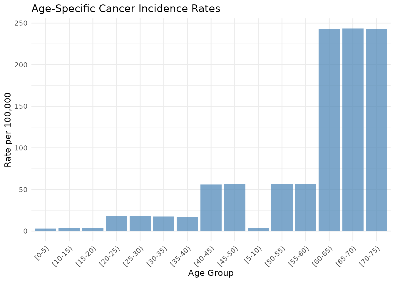
# Contribution to ASR plot
p2 <- ggplot(age_specific_data, aes(x = age_group, y = contribution_to_asr * 100000)) +
  geom_col(fill = "darkgreen", alpha = 0.7) +
  theme_minimal() +
  labs(
    title = "Contribution of Each Age Group to Age-Standardised Rate",
    x = "Age Group",
    y = "Contribution per 100,000"
  ) +
  theme(axis.text.x = element_text(angle = 45, hjust = 1))

print(p2)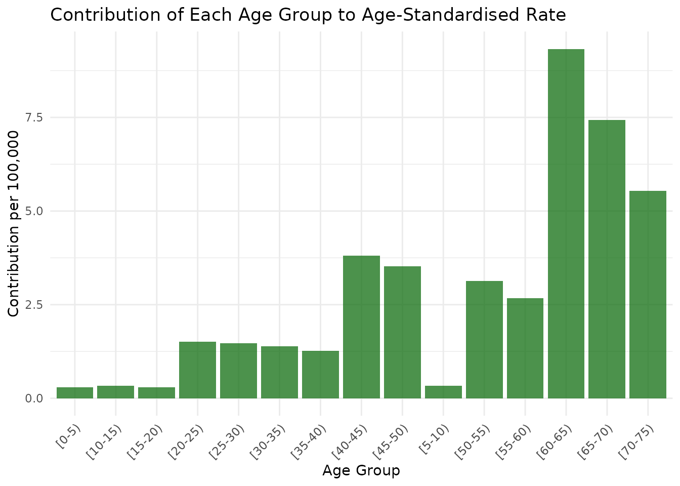
# Compare crude vs age-standardised rates
comparison_data <- data.frame(
  Rate_Type = c("Crude Rate", "Age-Standardised Rate"),
  Rate = c(cancer_asr$crude_rate_scaled, cancer_asr$asr_scaled),
  CI_Lower = c(NA, cancer_asr$asr_ci_lower_scaled),
  CI_Upper = c(NA, cancer_asr$asr_ci_upper_scaled)
)

p3 <- ggplot(comparison_data, aes(x = Rate_Type, y = Rate)) +
  geom_col(fill = c("orange", "purple"), alpha = 0.7, width = 0.5) +
  geom_errorbar(
    aes(ymin = CI_Lower, ymax = CI_Upper),
    width = 0.2,
    na.rm = TRUE
  ) +
  theme_minimal() +
  labs(
    title = "Crude vs Age-Standardised Cancer Incidence Rates",
    x = "Rate Type",
    y = "Rate per 100,000"
  )

print(p3)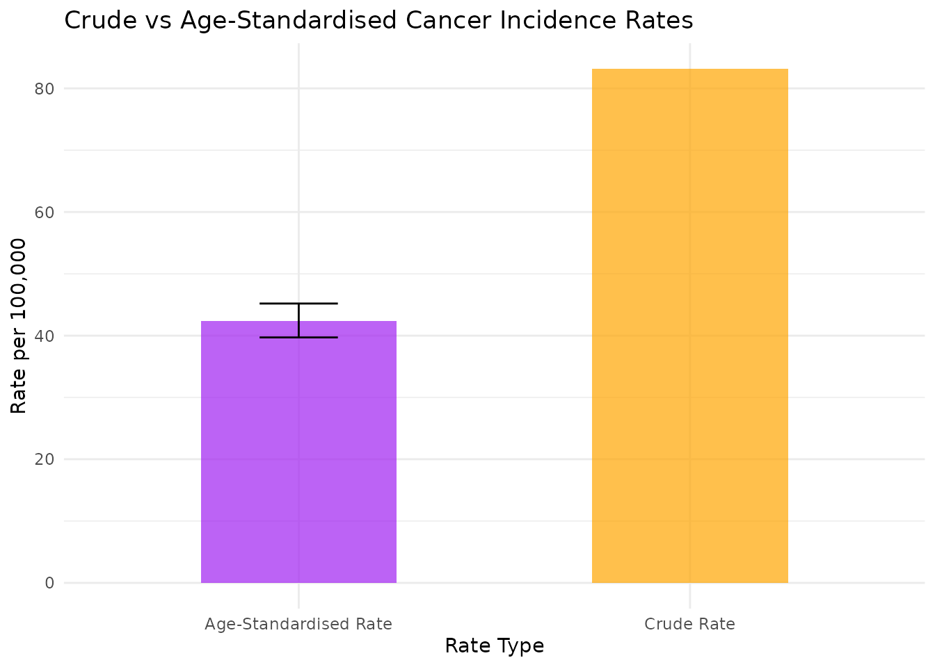
Example 4: Age-Standardised Prevalence Rates
The calculate_asr_direct() function can also be used to
calculate age-standardised prevalence rates. For prevalence studies, the
key differences are:
- events: Number of individuals with the condition at a point in time
- person_years: Total number of individuals examined/surveyed (use population counts, not person-years of follow-up)
- multiplier: Use 100 to express results as percentages (%) instead of rates per 100,000
# Example: Age-standardised prevalence of diabetes in a population survey
set.seed(789)

# Create synthetic diabetes prevalence data
diabetes_data <- data.frame(
  age_group = c("18-29", "30-39", "40-49", "50-59", "60-69", "70+"),

  # Number of individuals with diabetes (events)
  events = c(12L, 45L, 98L, 156L, 203L, 167L),

  # Total number of individuals surveyed in each age group (person_years = N individuals)
  person_years = c(1200, 1500, 1800, 1400, 1100, 800),

  # WHO standard population weights for corresponding age groups
  standard_pop = c(2435, 2021, 1826, 1485, 1118, 763)  # Simplified WHO weights
)

print("Diabetes prevalence survey data:")
#> [1] "Diabetes prevalence survey data:"
print(diabetes_data)
#>   age_group events person_years standard_pop
#> 1     18-29     12         1200         2435
#> 2     30-39     45         1500         2021
#> 3     40-49     98         1800         1826
#> 4     50-59    156         1400         1485
#> 5     60-69    203         1100         1118
#> 6       70+    167          800          763

# Calculate age-standardised prevalence using multiplier = 100 for percentages
diabetes_prevalence <- calculate_asr_direct(
  .df = diabetes_data,
  multiplier = 100,  # Use 100 to get percentages instead of per 100,000
  warn_small_cases = FALSE
)

print("Diabetes Prevalence Results:")
#> [1] "Diabetes Prevalence Results:"
print(paste("Crude prevalence:", round(diabetes_prevalence$crude_rate_scaled, 2), "%"))
#> [1] "Crude prevalence: 8.73 %"
print(paste("Age-standardised prevalence:", round(diabetes_prevalence$asr_scaled, 2), "%"))
#> [1] "Age-standardised prevalence: 7.42 %"
print(paste("95% CI:", round(diabetes_prevalence$asr_ci_lower_scaled, 2), "% -",
            round(diabetes_prevalence$asr_ci_upper_scaled, 2), "%"))
#> [1] "95% CI: 6.86 % - 8.01 %"

# View age-specific prevalence rates
age_specific_prev <- diabetes_prevalence$age_specific_data[[1]]
print("Age-specific prevalence rates:")
#> [1] "Age-specific prevalence rates:"
print(age_specific_prev[, c("age_group", "events", "person_years", "age_specific_rate_scaled")])
#>   age_group events person_years age_specific_rate_scaled
#> 1     18-29     12         1200                 1.000000
#> 2     30-39     45         1500                 3.000000
#> 3     40-49     98         1800                 5.444444
#> 4     50-59    156         1400                11.142857
#> 5     60-69    203         1100                18.454545
#> 6       70+    167          800                20.875000

# Plot age-specific prevalence
library(ggplot2)
p_prev <- ggplot(age_specific_prev, aes(x = age_group, y = age_specific_rate_scaled)) +
  geom_col(fill = "darkred", alpha = 0.7) +
  theme_minimal() +
  labs(
    title = "Age-Specific Diabetes Prevalence",
    x = "Age Group",
    y = "Prevalence (%)"
  ) +
  theme(axis.text.x = element_text(angle = 45, hjust = 1))

print(p_prev)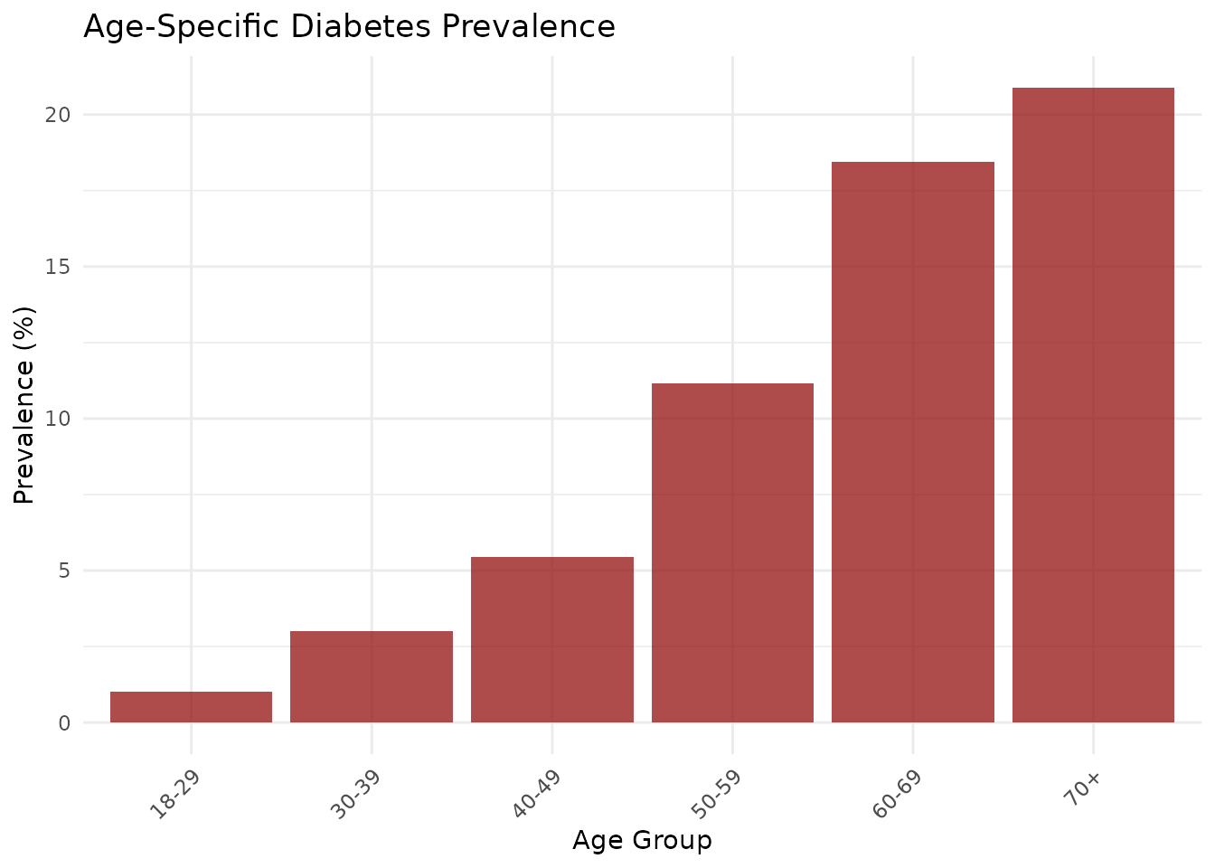
Key Points for Prevalence Studies:
- Cross-sectional data: Use counts of individuals with/without condition at a specific time point
- Population denominator: Use total number of individuals examined, not person-years of follow-up
-
Percentage scale: Set
multiplier = 100to express results as percentages (%) - Interpretation: Results represent the proportion of the population with the condition, standardised for age differences
Key Features Summary
calculate_person_years_by_age_strata()
- Calculates person-years of follow-up by age groups
- Default age groups now match WHO 2000-2025 Standard Population exactly
- Handles age transitions during follow-up period automatically
- Flexible age group definitions for custom analyses
- Final age group displays as “[100+)” to match WHO format
- Returns events and person-years by age strata
calculate_asr_direct()
- Calculates age-standardised rates using direct standardisation
- Works seamlessly with WHO age groups from person-years function
- Supports both incidence rates and prevalence calculations
- Two confidence interval methods: gamma distribution (default) and Byar’s/Dobson approximation
- Smart warnings for small/zero case counts with user control
- Returns comprehensive results including crude rates, ASRs, confidence intervals, and totals
WHO Standard Population Data
- Ready-to-use WHO 2000-2025 World Standard Population
- Multiple standard population formats available
- Easily integrates with the package functions
This vignette demonstrates the basic usage of the key functions in
epiUtils. For more detailed information about specific
functions, see their individual help pages.